From the Editor

Evaluating the assumptions of linear regression models

The purpose of linear regression is to describe the linear relationship between two variables when the dependent variable is measured on a continuous or near-continuous scale. For example, in the relationship between age and weight of a pig during a specific phase of production, age is the independent variable and weight is the dependent variable. As the pig’s age increases, its weight will also increase.

Many statistical tests are easy to apply to data because of computer software packages available today. With a drop-down menu, we select a statistical test and the computer applies the correct mathematical model and produces an output. If the P value of the test is less than. 05, we consider the association significant and publish the results. Why don’t you try this? Using Excel (Microsoft Corporation, Redmond, Washington) or another spreadsheet package, make two columns of data. The first column is parity and the values are 1, 1, 3, 3, and 3, representing two parity-one sows and three parity-three sows. In the second column, add litter size, represented by six, eight, 10, 12, and 12 pigs in each row, respectively. Then open the regression function and regress litter size on parity. The results suggest that litter size increases by 2.2 pigs as parity increases by one unit, and the P value is .03. Do you believe the results of this analysis? Does this data represent a linear relationship between parity and litter size? What if you were reading someone else’s results?

There must be quality control for all scientific tests. Each statistical test is based on fundamental assumptions. If the assumptions are violated, the results of the relationship described by the model are invalid. This is true even if the P value is < .05. Quality control for linear regression models is based on the diagnostics that we apply to the models to test the assumptions of the statistical test. If a published manuscript describes a model without describing the diagnostics applied to the final model, quality control is suspect. The results may or may not be valid. This may lead to a serious misinterpretation of the data and erroneous conclusions.

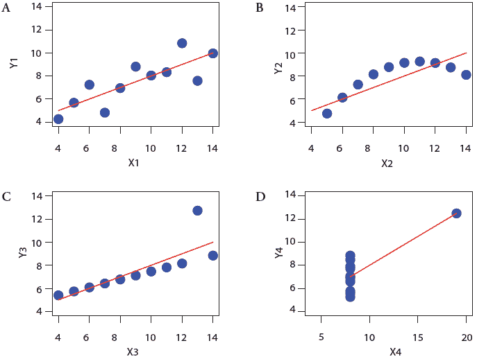
We will use a classical dataset known as Anscombe’s quartet,^1,2 illustrated by Figures 1A through D. In each graph, you see a scatterplot of the data points or the observations and the line representing the relationship between the two variables. The linear regression model estimates the least squares regression line, which is the line that minimizes the difference between the observed values and the predicted values. The models for all four data sets are the same, ie, the lines estimating the linear relationships between the independent and dependent variables are the same. Each line is defined by the regression coefficient; the intercept indicates where the line crosses the y-axis and the slope represents the angle of the line. Each line has the same test of statistical significance represented by the P value. Yet a simple visual inspection of the observations (blue dots) tells us that only the data in Figure 1A appears to accurately represent a linear relationship. We use these simple data sets to illustrate what is driving the estimated linear relationship in each of these figures. We will demonstrate how model diagnostics may be applied to determine whether or not the linear relationship is valid. In practice, and particularly in a multivariable model with several predictors, such plots of raw data may not be especially revealing, and we need to rely on model diagnostics to detect violations of the assumptions and to identify observations that have either a poor fit or an undue influence on the model.

Linear regression models assume that the residuals are normally distributed, that each observation is independent of the others, that there is a linear relationship between the independent and dependent variables, and that the variance of the dependent (outcome) variable does not change with the value of the independent variable. More details about the assumptions of linear regression models may be found elsewhere.^1-3 The major assumptions need to be evaluated, and fitting the best final model requires much more than simple one-step specification of a model and interpretation of summary statistics. It is an iterative process in which outputs at one stage are used to validate, diagnose, and modify inputs for the next stage.² Small violations of assumptions usually do not invalidate the conclusions. However, a large violation will substantially distort the association and lead to an erroneous conclusion.

Model assumptions are evaluated in two stages, looking first at the whole data set and then at individual observations. The first step is to calculate the residual for each observation. The residual is the numeric difference between the observed value that you entered into the data set and the predicted value derived from the model. Standardized residuals are calculated by dividing each residual by its standard error. These standardized residuals are plotted against the predicted values for the observations using a scatterplot (Figure 2A). If the assumption of equal variance over the values of the independent variable is true (homoscedasticity), then the scatter of points across the predicted values will form a band with no obvious decreasing or increasing pattern of residuals with increase in the predicted values. If the sizes of the residuals change as the values of the predicted outcomes changes, then we know that the assumption of equal variance is not true. This is a major violation of the linear regression. It will impact the calculation of the standard errors, which in turn will alter the size of the P value. This therefore would be a serious flaw in the assumptions.

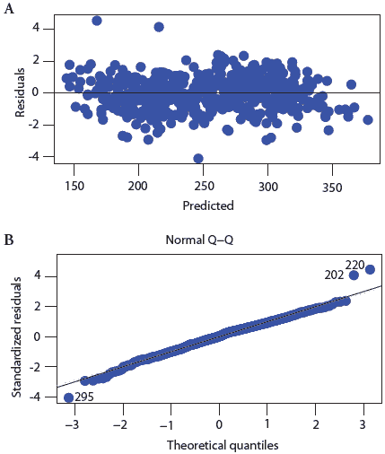
The assumption that the residuals are normally distributed is examined using a normal probability plot for the standardized residuals. If the assumption of normality holds, the standardized residuals will form a straight line with an intercept of zero and a slope represented by a 45° line (Figure 2B).

Independence of the observations means that they are not related to one another or somehow clustered. If some observations are taken from one farm and others from a different farm, then the observations are not independent. To “control” for this violation of the assumption, the farm of origin must be included in the model.

To test whether or not there is a linear relationship between the independent and dependent variables, we plot the standardized residuals against each independent observation. This can be illustrated using the observed data in a simple regression, as illustrated in Figures 1A through D, but for a multivariable model, we need to use the standardized residuals. In Figure 1B, the scatterplot indicates that there is a curvilinear rather than a linear relationship between the independent and dependent variables.

In the second stage of model evaluation, we use the residuals and other diagnostic statistics to identify outliers, leverage observations, and influential observations. Outliers are observations with “large” residuals compared to the other observations (Figure 1C), typically with standardized residuals < -3 or > 3. Leverage observations are cases with unusual “x” values (Figure 1D) and influential observations are cases with a large influence on the model (Figure 1C and D). These diagnostics give the researcher an opportunity to investigate whether or not the data is correct. Sometimes model diagnostics identify data input errors. Leverage indicates the potential of an observation to have an impact on the model. In the linear regression model, its value depends only on the predictor. The leverage value is high if the value of the observation is very far from the mean value of the independent variable, for example, if we added a parity-eight sow to the fictitious data set we created above. Cook’s distance and DFITS^2,3 are used to detect the influence of an observation on a model. Either a large residual or a large leverage can generate a large influence. Typically, we print out the values of these statistics for each observation and identify observations with unusual values relative to the others in the dataset. Applying these steps to the datasets in Figures 1C and 1D will identify violations of assumptions and other problems with the fitted models.

As we critically evaluate the literature, we must look to see that regression models are properly evaluated for quality to ensure that the assumptions have been met. If the model diagnostics are not performed, we cannot know whether or not the conclusions drawn from the model are valid.

References

1. Anscombe FJ. Graphs in statistical analysis. Amer Statistician 1973;27:17-21.

2. Chatterjee S, Hadi AS. Regression Analysis by Example. 4th ed. Hoboken, New Jersey: Willey-Interscience; 2006:375.

3. Dohoo I, Martin W, Stryhn H. Veterinary Epidemiologic Research. Charlottetown, Prince Edward Island, Canada: AVC Inc; 2003: 706.

-- Cate Dewey

-- Zvonimir Poljak